Turbidity
Turbidity is interpreted from satellite instrument observations. The data contains specifically the sea areas and lakes surrounding Finland. Observations are obtained during cloudless periods. In the maps, turbidity variations are described using a color map: clear water areas change to blue, in turbid areas the color changes from yellow to red, and especially turbid areas turn to purple. The background reference map is visible in areas with land, clouds, ice, or no observation. Turbidity maps often show natural variation, such as soil brought into the coastal waters by rivers or resuspension caused by strong winds, which raises more turbid water from the bottom to the surface. Turbidity maps often demonstrate how turbid water flows into estuaries through coastal rivers, especially during the melting season in spring and after heavy rains. Finnish lakes have highly variable levels of turbidity. In Tarkka, you can adjust the color map of the images if the variation in the lakes is not clearly visible with the default color map.
The turbidity interpretation is based on the reflection of solar radiation from the water area detected by the satellite instrument, which is high in turbid water areas. The interpretation of turbidity is done with a neural network-based model (C2RCC, Brockmann et al. 2016; Doerffer, et al. 2007; 2008a; 2008b). The model is used in various forms in several international services, such as Eumetsat and OC-CCI, which produce data for the world's marine regions. The model is openly available through SNAP software. In Syke's data, however, the final result of the model has been adapted to correspond more closely to the optical properties of the Finnish coast and lake areas (work done during the VESISEN project). The adaptation is based on field campaigns on the coastal riverine areas and statutory station sampling by the environmental administration of Finland (e.g. Attila et al., 2013).
The accuracy of the interpretation is good compared to turbidity samples collected from monitoring stations and laboratory analysed samples (depending on the region and reference data (r2 0.8-0.67), examples of data comparisons at the bottom of the page). When comparing turbidity observations at the water body level, the EO turbidity observations correspond well to the observations made at the stations (r2 = 0.76, RMSE = 3.2 FNU, MAE = 1.4, N = 286).
Since 2016, the interpretation has used the MSI instruments of the Sentinel-2 series of the EU Copernicus program and the observations of the OLI instrument of NASA's Landsat-8 satellite. An interpretation made with a spatial resolution of 60 m can be extended to archipelago and areas close to shoreline. High resolution observations are particularly beneficial in small-sized Finnish lake areas. The three currently available high resolution instruments have overpasses in Finland every few days.
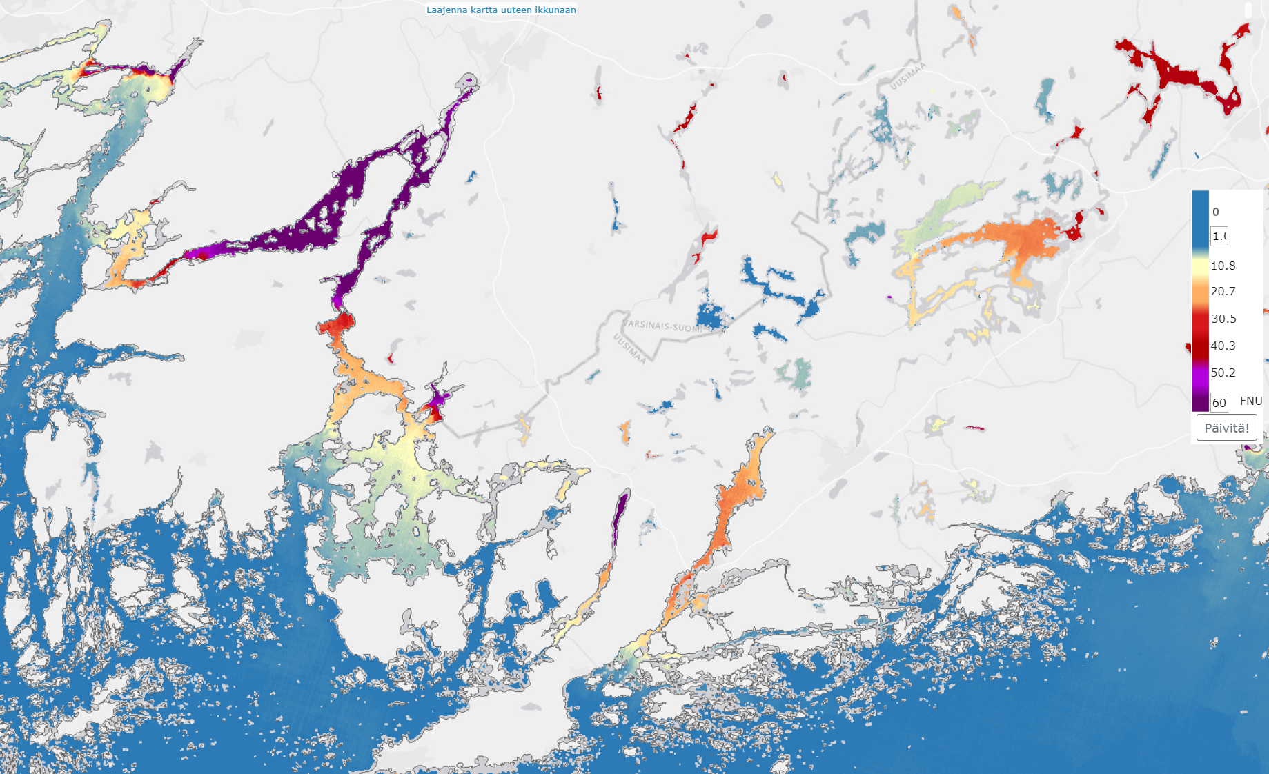
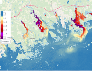
Example of turbidity data 07.04.2020, Sentinel-2 MSI. Contains Copernicus Data, Syke (2020).
For the years 2003-2011, the ENVISAT MERIS instrument's 300 m terrain resolution turbidity data will also be accurately updated, covering the entire Baltic Sea region, especially from the high seas. The turbidity interpretation for the MERIS period was based on an earlier version of the bio-optical model (C2R, Doerffer, et al. 2007; 2008a; 2008b). The calculation result of the bio-optical model has been adapted to correspond to the optical properties of the Finnish coast (Attila et al., 2013).
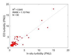
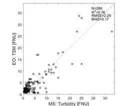
EO turbidity observations in comparison to monitoring station observations on the coastal waters of Finland. EO turbidity interpretation on coastal waters and on Finnish lakes.
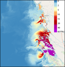
Examples of turbidity products on the coastal waters in the melting season in spring. On the left, the Kokemäenjoki River and the smaller estuaries to its north (14.4.2016), on the right, the areas from the Eastern Gulf of Finland (20.4.2019). Contains Copernicus Data, Syke (2019).
References
Attila, J., Koponen, S., Kallio, K., Lindfors, A., Kaitala, S., & Ylöstalo, P. (2013). MERIS Case II water processor comparison on coastal sites of the northern Baltic Sea, Remote Sensing of Environment, 128, 138–149.
Brockmann, C & Doerffer, R. (2016). Evolution of the C2RCC neural network for Sentinel 2 and 3 for the retrieval of ocean color products in normal and extremely optically complex waters. Proc. Living Planet Symposium, ESA SP-470.
Doerffer, R. & Schiller, H. (2007). The MERIS Case 2 algorithm. International Journal of Remote Sensing, 28 (3-4), 517-535. doi: 10.1080 / 01431160600821127.
Doerffer, R., & Schiller, H. (2008a). MERIS Regional Coastal and Lake Case 2 Water Project Atmospheric correction ATBD (Algorithm Theoretical Basis Document) 1.0. 41 pp. Http://www.brockmann-consult.de/beamwiki/download/attachments/1900548/meris_c2r_atbd_atmo_20080609_2.pdf
Doerffer, R. & Schiller, H., (2008b). MERIS Lake Water Project - Lake Water Algorithm for BEAM, ATBD (Algorithm Theoretical Basis Document) 1.0, 17 p.